Improving Redshift Spectrum’s Performance & Costs

Amazon Redshift Spectrum is a feature within the Amazon Redshift data warehousing service that enables Redshift users to run SQL queries on data stored in Amazon S3 buckets, and join the results of these queries with tables in Redshift.

Redshift Spectrum was introduced in 2017 and has since then garnered much interest from companies that have data on S3, and which they want to analyze in Redshift while leveraging Spectrum’s serverless capabilities (saving the need to physically load the data into a Redshift instance). However, as we’ve covered in our guide to data lake best practices, storage optimization on S3 can dramatically impact performance when reading data.

In this article, we will attempt to quantify the impact of S3 storage optimization on Redshift Spectrum by running a series of queries against the same dataset in several formats – raw JSON, Apache Parquet, and pre-aggregated data. We will then compare the results when it comes to query performance and costs.

The Data

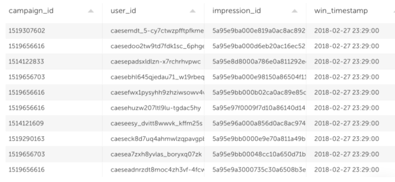
We used two online advertising data sets. The first dataset is ad impressions (instances in which users saw ads) and contains 2.3 million rows.

The second dataset is user clicks on ads – this data contains 20.2 thousand rows.

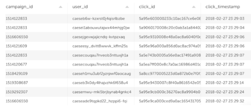
We uploaded the data to S3 and then created external tables using the Glue Data Catalog. When referencing the tables in Redshift, it would be read by Spectrum (since the data is on S3).

The Architecture

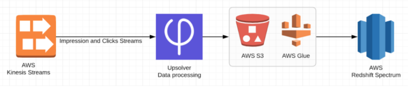
As we’ve explained earlier, we have two data sets impressions and clicks which are streamed into Upsolver using Amazon Kinesis, stored in AWS S3 and then cataloged by Glue Data Catalog for querying using Redshift Spectrum.

Data Ingestion, Storage Optimization and Data Freshness

As we’ve mentioned in the intro, Query performance in Redshift Spectrum is dramatically impacted by implementing data preparation best practices on the data stored in S3. You can find this in Amazon’s big data blog.

We wanted to benchmark this difference, both to show the impact of using Upsolver’s data lake ETL, and because manually implementing these best practices could be fairly complex and impact the time-to-production of your analytics infrastructure.

We ran our Redshift Spectrum queries on three different versions of the same original dataset:

• Compressed JSON files – each file contains 1 minute of data.
• An Upsolver Redshift Spectrum output, which processes data as a stream and automatically creates optimized data on S3: writing 1-minute Parquet files, but later merging these into larger files (learn more about compaction and how we deal with small files); as well as ensuring optimal partitioning, compression and Hive integration.
• An Upsolver Aggregated Redshift Spectrum output, which both processes data as a stream and creates optimized data on S3 (stored as compacted Parquet files) while also storing the table data by key instead of keeping the entire original data set. The aggregations are being updated as an event stream, which means the optimized data on S3 constantly up-to-date.

As you will see below, Redshift Spectrum queries on optimized data ran significantly faster, especially when in the case of 1-minute compacted Parquet files using Upsolver’s Redshift Spectrum output.

Since Redshift Spectrum charges $5 per terabyte of data scanned; we derived the costs you will see below from the amount of data each query needed to scan in order to return results.

The Results

We ran the SQL queries in Redshift Spectrum on each version of the same dataset. You can find the details below, but let’s start with the bottom line:

Redshift Spectrum’s Performance

• Running the query on 1-minute Parquet improved performance by 92.43% compared to raw JSON
• The aggregated output performed fastest – 31.6% faster than 1-minute Parquet, and 94.83% (!) faster than on raw JSON

The results validated our initial assumption, i.e. that data compaction (merging small files) and file formats play a major role when it comes to Spectrum query performance. When data is not compacted, Redshift Spectrum needs to scan a larger amount of files, and this slows down Spectrum. These results are very similar to what we saw in our Athena benchmarking tests.

We managed to further improve the results by creating aggregate tables using Upsolver. Those tables already contain all the needed aggregations which further cuts down the amount of data that needs to be scanned and processed, which improved both performance and costs.

Redshift Spectrum’s Costs

• Running the query on 1-minute Parquet improved costs by 34% compared to unaltered Parquet
• The aggregated output improved costs by 85% compared to 1-minute Parquet, and 90% compared to JSON

As we can see, the ‘knockout’ winner in this round would be the Upsolver aggregated output. This could be explained by the fact that Redshift Spectrum pricing is based on scanning compressed data.

Redshift Spectrum manages to scan much less data when the data is optimized to return the same query, with the end result being that running the same analytic workfload over optimized data would cost 90% less than on non-optimized data.

Query Performance

We will proceed to detail each query that we ran and the results we got from each version of the data sets.

Volume Distribution Per Campaign

SELECT campaign_id, count(id)

FROM [impressions table]

WHERE campaign_id IS NOT NULL

GROUP BY campaign_id;

Results:

Latency (seconds)       Data Scanned (MB)

JSON.                                    85                                     59.22

Parquet – Optimized          6                                     38.83

Parquet – Optimized &      4                                      1.23

Aggregated

CTR Calculation Per Campaign

SELECT i.campaign_id, CAST(((100.0*count(c.id)/NULLIF(count(*),0))) AS decimal(8,4) ) as CTR_calculation

FROM [Impressions table] i

LEFT OUTER JOIN [Clicks table] c ON i.id = c.id

GROUP BY i.campaign_id;

Results:

Latency (seconds)                  Data Scanned (MB)

JSON                                    79                                                64.63

Parquet – Optimized.         9                                                  41.86

Parquet – Optimized &      7                                                   1.05

Aggregated

Top 5 Fraud Candidate Users (With The Highest Impressions)

SELECT exch_user as user_id, count(id) as impressions_count

FROM [Impressions table]

GROUP BY user_id

ORDER BY 2 desc

limit 5;

Results:

Latency (seconds)           Data Scanned (MB)

JSON                                            87                                        59.22

Parquet – Non Optimized         4                                          37.14

Parquet – Optimized &              2                                          14.72

Aggregated

Next steps

Want to learn more about optimizing your data architecture? Check out the following resources:

• Amazon Athena and Google BigQuery Benchmarks
• Amazon Athena vs traditional databases
• Principles for data lake architecture
• Get a live demo fo Upsolver
• Try SQLake for free (early access). SQLake is Upsolver’s newest offering. It lets you build and run reliable data pipelines on streaming and batch data via an all-SQL experience. Try it for free. No credit card required.