Using Upsolver to Flatten JSON Arrays into Athena Tables

Dealing with arrays and nested objects so as to make the data usable comes with the territory: 

• Some target systems won’t support arrays or nested objects; you must flatten and clean up the data before you output it to them. 
• Some systems do support arrays or nested objects natively.  However:
  • working with these systems can be difficult and affects data access.  Flattening the data ahead of time – that is, before querying it – removes this burden.   
  • you still must account for arrays when the values are calculated and the data is enriched.  Otherwise, the system could mix up values and return incorrect results.

Flattening the data maximizes its usability.  But it’s difficult to use SQL to process this data such that it’s fully available to query engines.  You can do it manually with code – identify the object, understand its syntax, possibly relate it to other arrays, write the code for it, then test it out.  But this doesn’t scale.

Nor can you avoid dealing with these objects.  Some of your producers who provide data with arrays may be beyond your direct control.  Some data producers who are beyond your direct control may provide data with arrays.  And in any case, if you’re working with multiple streaming data sources, whether from document DBs, event streams, services such as Kafka or Kinesis, and so on, there’ll likely be complex objects – arrays with items, classes, categories, and so on – in there somewhere.  If you lack good visibility into the data coming in, you may not even know they’re there. 

What’s needed is a robust default handling behavior for arrays.  That’s what Upsolver provides. 

Upsolver supports arrays natively.  It removes the need for manual review and intervention, automating all of the steps involved and also handling all behind-the-scenes processing.  That includes calculations on fields originating from arrays; in this case Upsolver uses the target field name of calculations to determine how to proceed. 

Here’s an example of how straightforward this can be using Upsolver: 

• ingesting nested data that contains arrays, 
• sending it to Athena for data analysts to investigate and derive business insights.  When you do this Upsolver automatically flattens the arrays out by line item.

In the following specific example we work with retail store sales data, which the data team wants to analyze to determine the company’s best-performing items and stores.  But the concept of flattening arrays, and Upsolver’s automated method of addressing it, spans industries and use cases.

Creating a Data Source for Ingestion

We begin, as we always do with Upsolver, with a data source.  Upsolver can bring data in from almost any source:

• files (Hadoop, Amazon S3, Azure storage)
• streams (Kinesis, Kafka, event hubs, or virtually any streaming solution)
• relational databases (e.g. CDC)

In this particular instance, S3 is the data source.  When you select your data source, Upsolver immediately detects and previews the data it contains, so you can verify it is in fact what you seek.  If you wish, you can also create a new folder to house the data.

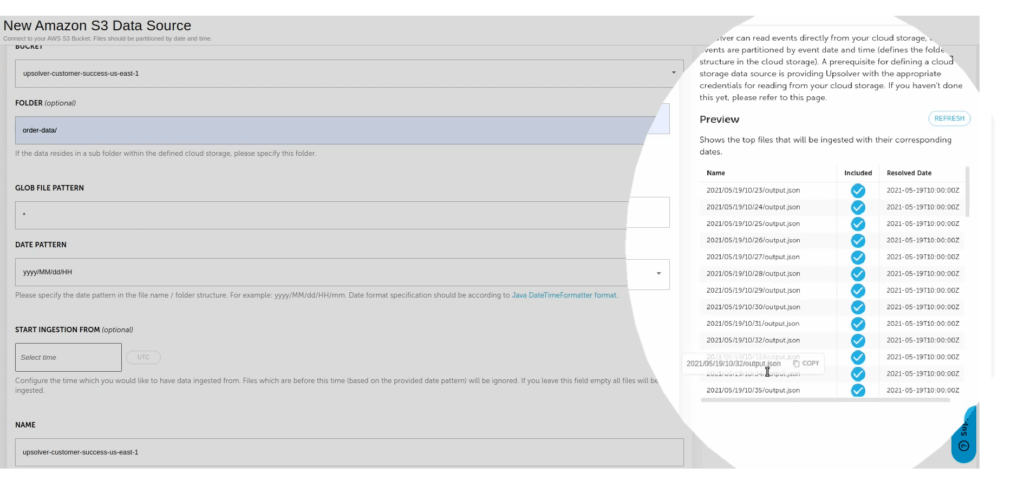
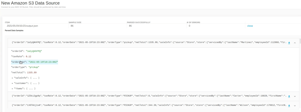
Continue, and Upsolver automatically detects the source file format – in this case, JSON – and the compression method used.  Then it displays the files, on which you can drill down to confirm you’ve got the desired set of data – in this case, data on store sales (order information, store location, and so on). 

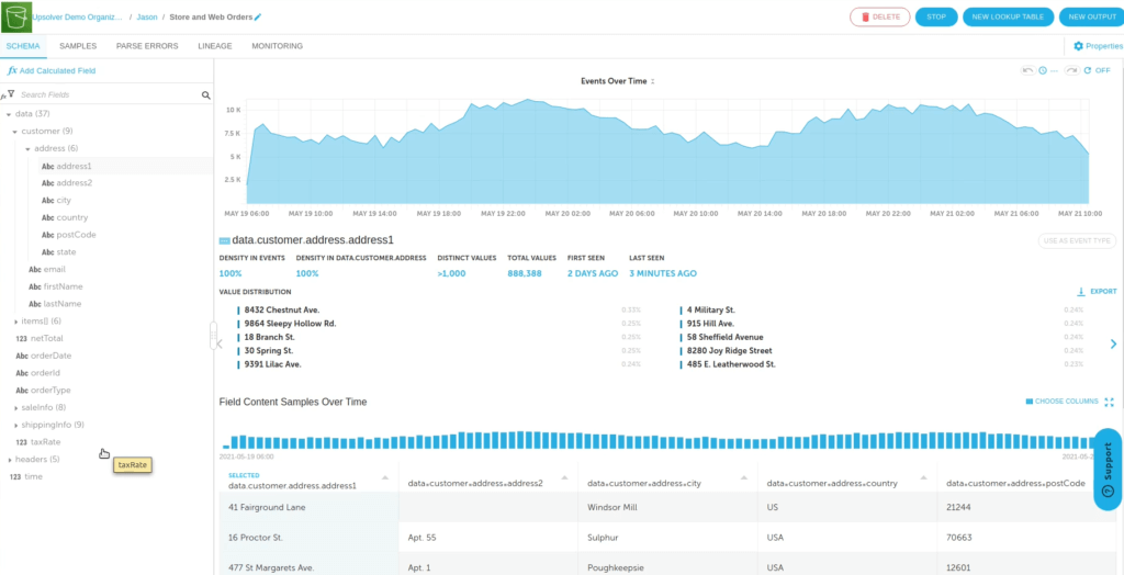
Click Create.  Upsolver displays a wide range of statistics about the data including, in the lefthand side, the various fields.  This schema-on-read method enables Upsolver to detect new fields and add them automatically to this list.  It also removes from your responsibility the onerous job of managing fields explicitly.

As for the statistics, you can explore a comprehensive set of metadata per each field, such as:

• Density (is the field fully-populated with values?)
• Distinct values
• Time period

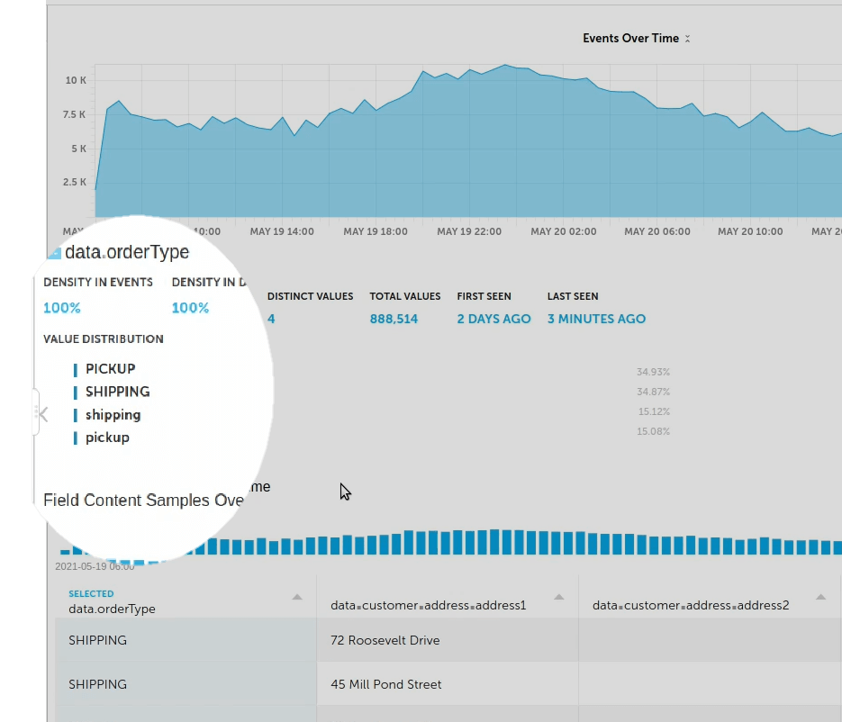
Among other things, you can use these statistics to check for data integrity, or to identify errors or issues early in the process, before they cause problems downstream.  In this example, there’s a case discrepancy – the orderType field displays shipping and pickup in both upper case and lower case – and you can address this before sending the data to Athena, where it could impact the results.

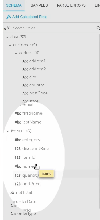
You can also view nested data – specifically in this case, an array of elements under the item field, where there may be multiple items per purchase order.  This is the data you must flatten – item name, unit price, quantity, and so on – before you can output it for analysis by Athena.  The intent here is to create a table that combines item and store information and gain insight into which items perform best by country and store.

The next step is to begin creating your output.  Upsolver prompts you for a destination. Here it’s Athena, although Upsolver provides many options:

• Data warehouses such as Redshift or Snowflake
• Batches of files in a data lake
• Query engines

Regardless of which target you choose, the process in Upsolver is the same.

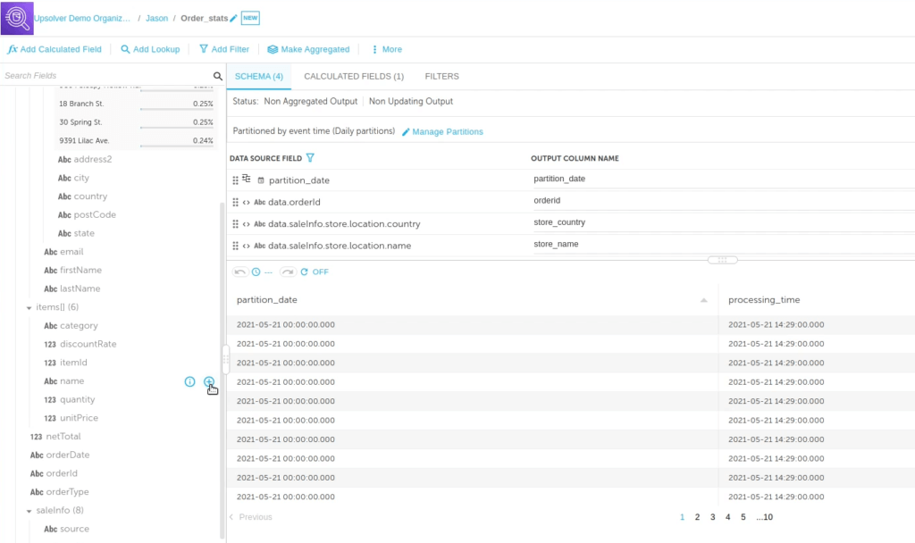
Name your output and click Next.  On the lefthand side Upsolver displays all the fields available in your data source; on the right it displays the columns to add to the Athena table you want to create.  Again, preview the data.  From here you can remove any columns you don’t want, and add in any fields you do.  In this case, to obtain the analysis you want (item performance by store and country), add the orderID, the store_country, and the store_name.  And you can re-name the columns for your new table; you’re not required to use the field name in the source data.

Preparing an Array for Flattening Before Sending to Athena

Now add item information.  Here’s where you encounter an array.  When you attempt to add an array, Upsolver prompts you either to:

• Concatenate the values
• Specify a value (First element / Last element)
• Flatten the data source and write to a database.  This creates a new table row for each element common across all items in the array, and duplicates it across multiple rows – in essence, mapping items from the data source to the output table.

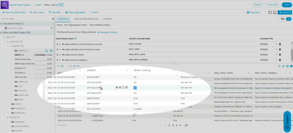
Click Flatten.  Then finish adding any other desired fields (in this case, items_name and items_category).  When you’re done, click Preview.  Again Upsolver displays your data, at which point you see multiple rows per orderID, indicating a discrete row per array element.

You can also create calculated fields – in this case, multiplying the unit price by quantity to get the final sale price.  Simply click Add Calculated Field, select from about 200 built-in mathematical and higher-level (such as geo_IP parsing) functions, and indicate your operant fields.

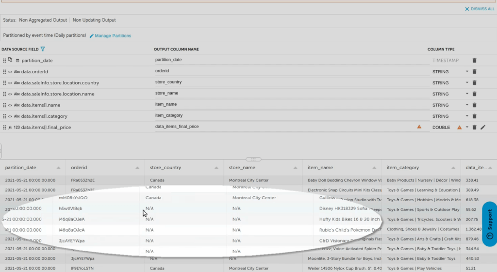
Be sure to place the result – the new, calculated field containing the result – within the corresponding data source field – in this case, final_price.  This preserves the context of the data, places the calculated result within the original array, and ensures that Upsolver calculates the correct results.  Upsolver flattens the data after the transformations and calculations to ensure you get the proper final price for each line item.

Click Save to preview the data once again.  Your new calculated field is added to the schema.

Filtering a Flattened Array and Deploying it to Athena

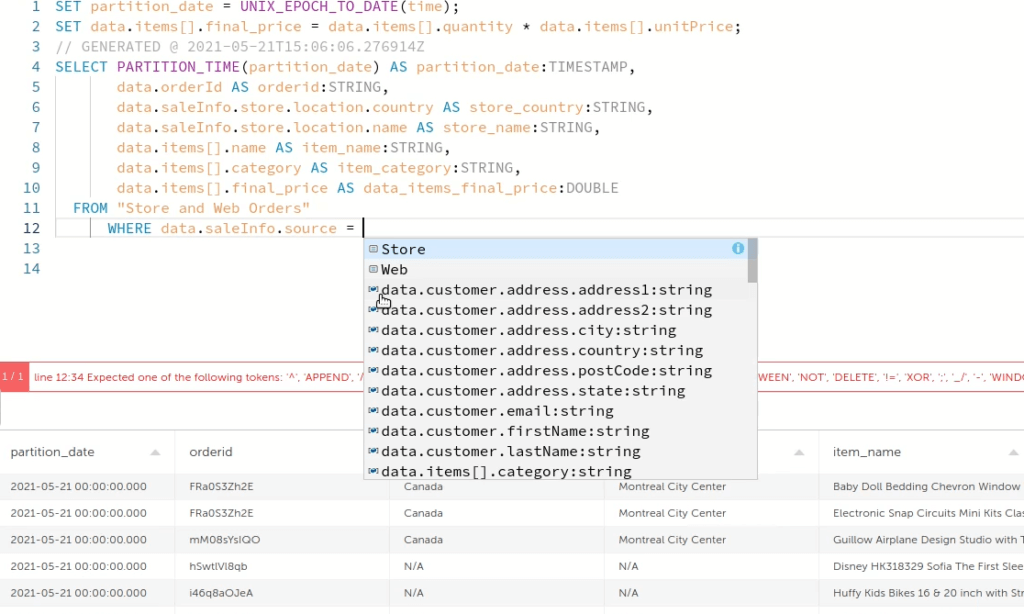
When you preview the data at this point you might observe there is data missing.  The reasons for this are contextual; in this case, one of the aggregated fields is available only for orders placed in physical stores – not online – so the rows indicating Web sales display with null values.  To rectify, simply apply a WHERE filter to send only physical store data to Athena. 

Throughout this process we’ve focused on the Upsolver GUI, and you can apply the WHERE filter via the GUI as well.  But if you prefer working directly in SQL or just wish to review the SQL code, now or at any time you can toggle back and forth between the GUI and SQL.  These two views sync in real-time, so regardless of when you toggle you always have the most recent view.  

Apply the filter and click Preview again to filter out all of the null values.  (Note that when you create a WHERE filter in the SQL view, Upsolver displays an auto-complete box that lists all of the field values; click the value you want to complete the filter.)

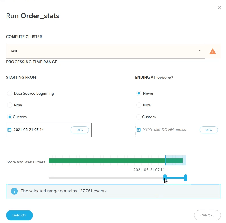
Now it’s time to deploy your code.  Click Run, enter the parameters when prompted (the storage bucket, the Athena table name, and so on), and click Next.  Specify the date range for the data you wish to query.  Obviously, the wider the date range, the longer before the data is fully available.  For a streaming output, for the Ending At option click Never.  That instructs Upsolver to continually append new data to the table as the data arrives.  Latency typically is ~1 minute.

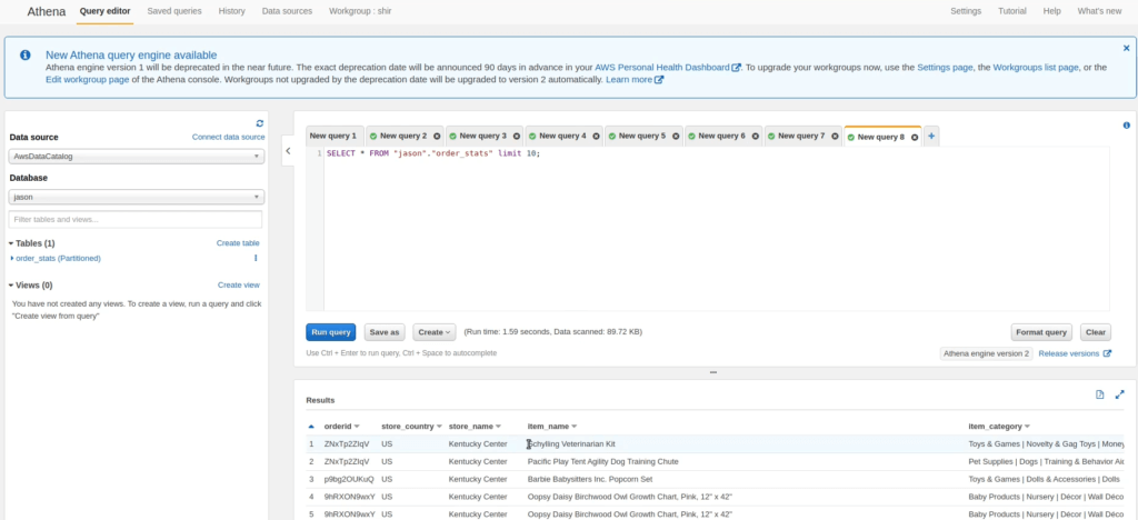
Click Deploy.  Upsolver automatically creates the Athena table.  Open Athena.  The table you just created displays.  Run the query and view your results.  This query is now available to any of your data practitioners, and it always contains the freshest data. 

What we’ve just illustrated is a very simple example.  But the process applies pretty much regardless of the complexity of your use case, or the number of arrays involved.  Upsolver automatically validates your algorithm.  If the default flattening could create a Cartesian Product, Upsolver displays a warning and gives you tools that enable you to specify relationships between array values.

Learn more about how Upsolver SQLake simplifies working with nested data.